1. Introduction
This document is for NANDRAD and SIM-VICUS developers. It discusses coding guidelines/rules and covers the underlying concepts of the solver and user interface implementation.
2. General Information
2.1. Building the code
Building the code is fairly easy and only requires two steps:
-
setup the development environment
-
run the build scripts
For actual development we recommend use of Qt Creator with the prepared qmake build system.
|
If you are serious with own development of SIM-VICUS/NANDRAD I strongly suggest using Linux and Qt Creator - building the code on Linux is way faster than on Windows/Mac, and code insights and clang analysis in Qt Creator (including refactoring features) are much much better than in Visual Studio and/or XCode. But that’s just my humble opinion after a "few" years of working with all of these :-) |
2.1.1. Setting up the build environment
Generally, you need a fairly up-to-date C/C++ compiler (that means: c++11 features should be supported). Also, you need the Qt libraries. And you need cmake. That’s it, nothing else!
Windows
There are build scripts for different VC and Qt versions. To keep things simple, all developers should install the same VC and Qt versions on development machines.
|
Team development works best if all use the same compilers and library versions. If you change build scripts and commit them to the repository, always make sure that you do not disrupt other peoples work by requiring alternative installation directories/tool versions. |
Required versions:
-
Visual Studio 2019 (Community Edition suffices)
-
Qt 15.5.2
Installation steps:
-
Download and install Visual Studio 2019 Community Online Installer from: https://visualstudio.microsoft.com/de/thank-you-downloading-visual-studio/?sku=Community&rel=16# - Once downloaded, you only need to install basic development options.
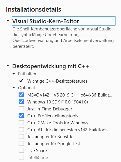 Figure 1. Minimal selection of Visual Studio components to be installed
(Profiling tools are optional, profiling can be done very well with
valgrindon Linux). -
Download and install cmake. Either download from https://cmake.org or use chocolatey (https://chocolatey.org) and run
choco install cmake
-
Download and install JOM (newer versions of the Qt maintenance tool do no longer install JOM together with QtCreator). Either download from https://cmake.org or use chocolatey (https://chocolatey.org) and run
choco install jom
-
Download and install Qt Online Installer (https://www.qt.io/download-qt-installer) and in the installation program select the 5.15.2 variant.
-
Download the VC Qt Tools addin (not really necessary for command line builds, but just in case you want to do development in VC directly - though I wouldn’t recommend it): https://marketplace.visualstudio.com/items?itemName=TheQtCompany.QtVisualStudioTools2019
Also, install a suitable git client (SmartGit is recommendet). Don’t forget to specify your git user name and email (user settings).
Linux
On Linux it’s a walk in the park. Just install the build-essential package (g++/clang and cmake and qt5default packages). On Ubuntu simply run:
> sudo apt install build-essential cmake qt5-default libqt5svg5-dev git qtcreator
Also, install git or a suitable git client (SmartGit is recommendet). Don’t forget to specify your git user name and email:
> git config --global user.name "Your name here"
> git config --global user.email "your_email@example.com"
|
On Ubuntu 18.04 LTS the default Qt version is 5.9.5, so that is the oldest Qt version we are going to support. Whenever deprecated features are used to maintain compatibility with Qt 5.9.5, and where newer Qt features are available in more recent versions of Qt, the use of |
MacOS
|
HomeBrew does no longer work well for older MacOS versions, such as El Capitan. You may have problems installing certain tools. However, you may still use it to install newer gcc versions, needed for parallel builds. Homebrew can be used to install other programs (see https://brew.sh). Then > brew install cmake |
On El Capitan (MacOSX 10.11) Qt 5.11.3 is the last version to work. So you need to manually download this version. First select the Qt online installer (https://www.qt.io/download-qt-installer) and select version 5.11.3. This ensures that all developers use the same Qt version and avoid Qt-specific compilation problems.
Parallel gcc OpenMP code require a bit of extra work (to be documented later :-)
Also, install git or a suitable git client (SmartGit is recommendet). Don’t forget to specify your git user name and email:
> git config --global user.name "Your name here"
> git config --global user.email "your_email@example.com"
2.1.2. Building
This works pretty much the same on all platforms. If you’ve successfully installed the development environment and can build basic Qt examples (open Qt Creator, pick an example, build it), you should be ok.
Go to the build/cmake subdirectory and run:
> ./build.sh
for Linux/MacOS or
> build_VC2019_x64.bat
or > build_VC2019_x64_with_pause.bat
for Windows.
On Linux/MacOS you can pass a few command line options to adjust the build, for example:
> ./build.sh 8 release omp
to compile in parallel with 8 CPUs and create a release build (optimized, no debug symbols) with OpenMP enabled. See the documentation in the build.sh script for more information.
Once the build has completed, the executables are copied into the bin/release (or bin/release_x64 on Windows) directory.
On Windows, you may want to run bin/release_x64/CreateDeploy_VC2019.bat batch file to fetch all required DLLs (so that you can start the application by double-clicking the executables).
|
In case of build problems, inspect the build scripts and the path variables therein. You may need to set some environment variables yourself before running the scripts. |
2.1.3. Development with Qt Creator
Development is best done with Qt Creator (it is way more efficient to work with than Visual Studio or Emacs/VI). The source code is split into many different libraries and executables, so you best open the prepared session project file build/Qt/SIM-VICUS.pro.
If you start working with Qt Creator, please mind the configuration rules described in Qt Creator Configuration.
2.1.4. Development with Visual Studio on Windows
To avoid the overhead of maintaining yet another build system (so far we have qmake/Qt Creator and cmake), we do not have Visual Studio solutions or project files. However, with the help of cmake you can easily generate VC project files for analysis of the code in Visual Studio.
Open a Visual Studio command line, ensure that cmake is in the path and then change into the SIM-VICUS/build/cmake directory. There, create a subdirectory, for example vc, change into this subdir, and run cmake.
Here are the commands when starting from within SIM-VICUS/build/cmake:
:: run from SIM-VICUS\build\cmake

:: load VC compiler path
"C:\Program Files (x86)\Microsoft Visual Studio\2019\Community\VC\Auxiliary\Build\vcvars64.bat"

:: set CMAKE search prefix to find Qt library
set CMAKE_PREFIX_PATH=C:\Qt\5.15.2\msvc2019_64

:: create a subdirectory 'vc' and change into it
mkdir vc
cd vc

:: generate cmake build system files
cmake -G "Visual Studio 16 2019" -A x64 ..
This generates build system files for Visual Studio 2019 64-bit.
|
If you have a different version of Visual Studio installed, use the respective project file generator as described in cmake-vc-generators |
The command will generate a set of *.vcproj files and an sln file:
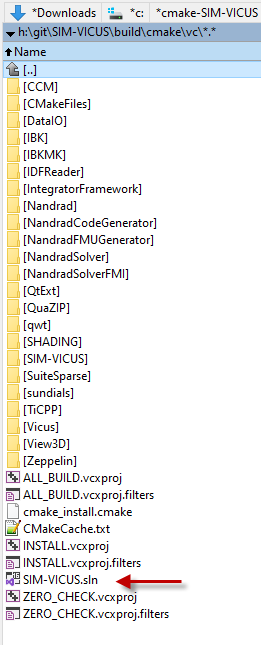
You can open that and start developing in VC. Just mind that you may need to update your project files whenever new files have been added to the SIM-VICUS source code.
|
Even if you’ve used Visual Studio in the past, we strongly advise against using it for SIM-VICUS development. The learning curve for Qt Creator is short and you will be rewarded with much better refactoring/code analysis features, plus much faster user interface (just try out the code completion!). Though, Visual Studio has it’s benefits when it comes to specific debugging tasks in the internals of the solver. |
2.2. Coding Guidelines and Rules
Why coding guidelines and rules?
Well, even if you write software just for yourself, once the code base reaches a certain limit, you will appriciate well written code, so that you:
-
avoid wasting time looking for variables, types, functions etc.
-
avoid re-writing similar functionality, simply because you don’t rememeber/find the already existing code pieces
-
avoid accidentilly breaking code because existing code is hard to read
Bottom line:
Write clean and easy to read and maintain code, both for yourself and others in the team.
The big question is: What is clean and easy to read/maintain?
Well, in my humble opinion this is mostly achieved by
-
doing stuff (mostly) the same way as everywhere in the code
-
using conventions that makes it easy to exchange code with others
-
using conventions that save you the trouble of remembering each and every variable/function etc.
-
write code that makes it easy for your development environment to assist you (see also section Qt Creator below)
Below I’ve collected a bunch of rules/guidelines that help us achieve this goal of getting nice code, without restricting the individual coding style of each developer too much.
2.2.1. Programming efficiency
We are a small team and need to get the most out of our programming time.
Basic rule: Know your tools and choose the right tool for the job!
For programmers, you need a good text editor (for everything that’s not actual code, or for quick hacks) and a decent development environment (IDE). I’d say Qt Creator wins big time against Visial Studio, XCode and any other stuff out there, but let’s not start an emacs vs. the world flame war here :-).
Of course, you also need to handle svn/git, diff and merge tools etc. but text editor and IDE are the most important. I’d suggest SmartGit as git client - not because it is the best out there, but because most of the team members use it and can help you better with a problem.
Knowing the capabilities of your particular IDE you can write code such, that already while typing you can use auto-completion to its maximum. This will speed up your coding a lot and save you much unnecessary compilation time. With code-checking-while-typing (see clang checks in Qt Creator), you’ll catch already 80% of typical compiler bugs, so we should use this.
Also, some of the naming conventions below help in an IDE to be fast, for example the m_ prefix in member variable names, really speed up coding. You need to access a member variable: type m_ and you’ll get only the member variables in the auto-completion, no mistake with local variables is possible.
2.2.2. Indentation and line length limit
-
only tabs for indentation, shown in display as 4 spaces - especially on larger monitors with higher resolutions this will allow you to see indentation levels easiy; and since we are using tabs, you may still switch your development environment to use 2 or 8 spaces, without interrupting other author’s code look
-
line length is not strictly limited, but keep it below 120 (good for most screens nowadays)
2.2.3. Character encoding and line endings
-
Line endings LR (Unix/Linux) - see also git configuration below
-
UTF-8 encoding
2.2.4. File naming and header guards
-
File name pattern:
<lib>_<NameInCamelCase>.*, for example:IBK_ArgsParser.horNANDRAD_Project.h -
Header guards:
#ifndef <filenameWithoutExtension>H, example:#ifndef NANDRAD_ArgsParserH
|
Rationale When header guards, filenames and class names use all the same strings (case-sensitive same strings), this makes refactoring a lot easier! And refactoring is something we need to do quite often. For example, if you need to fix a spelling mistake in: and similar for |
2.2.5. Namespaces
Each library has its own namespace, matching the file prefix. Example: NANDRAD::Project get NANDRAD_Project.h
|
Never ever write This is mostly a precaution, as in larger projects with many team members it is very likely that function names are similar or even the same, if written by different authors. When typing in your favourite development environment with code completion you are forced to write the namespace and the auto-completion will now only offer those functions/variables that are defined in the respective namespace (making it much harder to mistakely call a function you didn’t intend to call). |
2.2.6. Class and variable naming
-
camel case for variable/type names, example:
thisNiceVariable -
type/class names start with capital letter, example:
MyClassType(together with namespace prefix nice for auto-completion of type names) -
member variables start with
m_, example:m_myMemberVariableObject(useful for auto-completion to get only member variables) -
getter/setter functions follow Qt-Pattern:
Example:
std::string m_myStringMember;

const std::string & myStringMember() const;
void setMyStringMember(const std::string & str);|
Never ever write |
The reason for having strict rules for these access functions is two-fold:
-
you do not need to remember the actual names for the getter/setter functions or the variable itself - knowing one will give you the name of the others (less stuff to remember)
-
efficiency: you can use the Qt-Creator feature → Refactor→Add getter/setter function when right-clicking on the member variable declaration
2.2.7. Suggestions for writing clean and neat code
// Short function declarations may have the { in the same line
void someFunction(int t) {
    // indent with one tab character
    for (int i=0; i<t; ++i) { // also place the opening brace in this line
        // code
    }
    // longer for-clauses with more than one line should place
    // the opening { into the next line to mark the opening scope.
    for (std::vector<double>::iterator it = m_localVec.begin();
        it != m_localVec.end(); ++it)
    {
        // code
    }
    // similar rules apply for if and other clauses, for example
    if (value == 15 || takeNextStep ||
        (firstStepCounter > 15 && repeat))
    {
        // code
    }
}

// Longer function declarations in two or more lines should place
// the { in the next line to clearly mark the start of the scope.
void someFunctionWithManyArguments(const std::vector<double> & vec1,
    const std::vector<double> & vec2,
    const std::vector<double> & vec3)
{
    // code
}


// The following source code shows typical indentation rules
void indentationAndOtherRules() {

    // recommendation: use 'if (' instead of 'if( '
    if (someCondition) {
        // code
    }
    // put else in a separate line and put code comments
    // like this before the else clause to document what's
    // done in the else block
    else {
       //
    }

    // put spaces between ; separated tokens in for loops
    for (i=0; i<20; ++i) {
    }

    // indent switch clauses like the example below
    switch (condition) {
         case Well:
             // code
             // more code
         break; // break on same level as case

         // document case clauses before the case
         case Sick:
             // code
         return "sick";

         // when you declare local variables within switch
         // open a dedicated scope
         case DontKnow: {
             int var1;  // local variable, only valid for case clause
             // code
         }
         break;

         // if you have many short case clauses, you can use properly indented one-line versions
         case ABitSick        : return "a bit sick";
         case ALittleBitSick  : return "a little bit sick";
         case QuiteWell       : break;

         default: ; // only implement the default clause, when needed.
                    // Otherwise compiler will remind you about forgotten clauses
                    // (which might be quite helpful).
    } // switch (condition)
    // in long nested scopes, document the end of the scope as done in the line above

    // another example of documented nested scopes
    for (k=0; k<10; ++k) {
        for (j=k; j<10; ++j) {

            // lots of code

        } // for (j=k; j<10; ++j)

    } // for (k=0; k<10; ++k)
}
2.2.8. Enumeration types
Generally, enumeration types shall be named just as class names, that is using camel-case.
enum ModelType {
  MT_Standard,
  MT_MoreComplicated,
  MT_ReallyReallyDifficult,
  NUM_MT
};
The individual enum values shall use camel-cased names, and a prefix that is composed of initials of the actual enum type. This assists while typing, since one can just write "MT_" and will get the list of accepted enum types in the autocompletion list (avoids mixing enum value programm errors).
Add the NUM_MT enumeration value if keyword list support is needed (see documentation of code generator).
For keyword-list enums for parameters, integer parameters and flags there is the convention to use:
enum para_t {
  P_XXX,
  ...
  NUM_P
};

enum intPara_t {
  IP_XXX,
  ...
  NUM_PI
};

enum flag_t {
  F_XXX,
  ...
  NUM_F
};
This is a legacy naming that is just used everywhere in the code and best kept this way (never touch a running system :-)
2.2.9. Exception handling
Basic rule:
-
during initialization, throw
IBK::Exceptionobjects (and onlyIBK::Exceptionobjects in all code that uses the IBK library) : reason: cause of exception becomes reasonably clear from the exception message string and context and this makes catch-and-rethrow-code so much easier (see below). -
during calculation (in parallel code sections), avoid throwing Exceptions (i.e. write code that cannot throw); in error cases (like div by zero), test explicitely for such failure conditions and leave function with error codes
When throwing exceptions:
-
use function identifier created with
FUNCID()macro:
void SomeClass::myFunction() {
    FUNCID(SomeClass::myFunction);

    ...
    throw IBK::Exception("Something went wrong", FUNC_ID);
}
Do not include function arguments in FUNCID(), unless it is important to distinguish between overloaded functions.
When raising exceptions, try to be verbose about the source of the exception, i.e. use IBK::FormatString:
void SomeClass::myFunction() {
    FUNCID(SomeClass::myFunction);

    ...
    throw IBK::Exception( IBK::FormatString("I got an invalid parameter '%1' in object #%2")
        .arg(paraName).arg(objectIndex), FUNC_ID);
}
See documentaition of class IBK::FormatString (and existing examples in the code).
Exception hierarchies
To trace the source of an error, keeping an exception trace is imported. When during simulation init you get an exception "Invalid unit ''" thrown from IBK::Unit somewhere, you’ll have a hard time tracing the source (also, when this is reported as error by users and debugging isn’t easily possible).
Hence, if you call a function that might throw, wrap it into a try-catch clause and throw on:
void SomeClass::myFunction() {
    FUNCID(SomeClass::myFunction);

    try {
        someOtherFunctionThatMightThrow(); // we might get an exception here
    }
    catch (IBK::Exception & ex) {          // we can rely on IBK::Exception here, since nothing else is allowed in our code

        // rethrow exception, but mind the prepended ex argument!
        throw IBK::Exception(ex, IBK::FormatString("I got an invalid parameter '%1' in object #%2")
            .arg(paraName).arg(objectIndex), FUNC_ID);
    }
}
The error message stack will then look like:
SomeClass::someOtherFunctionThatMightThrow    [Error]           Something went terribly wrong.
SomeClass::myFunction                         [Error]           I got an invalid parameter 'some parameter' in object #0815
That should narrow it down a bit.
2.2.10. Documentation
Doxygen-style, prefer:
/*! Brief description of function.
    Longer multi-line documentation of function.
    \param arg1 The first argument.
    \param temperature A temperature in [C]
*/
void setParams(int arg1, double temperature);

/*! Mean temperature in [K]. */
double m_meanTemperature;
Mind to specify always physical units for physical value parameters and member variables! Physical variables used for calculation should always be stored in base SI units.
2.2.11. Git Workflow
Since we are a small team, and we want to have close communication of new features/code changes, and also short code-review cycles, we use a single development branch master with the following rules:
-
CI is set up and ensures that after each push to origin/master the entire code builds without errors - so before pushing your changes, make sure the stuff builds
-
commit/push early and often, this will avoid getting weird merge conflicts and possibly breaking other peoples code
-
when pulling, use rebase to get a nice clean commit history (just as with subversion) - makes it easier to track changes and resolve errors arising in a specific commit (see solver regression tests)
-
before pulling (potentially conflicting) changes from origin/master, commit all your local changes and ideally get rid of temporary files → avoid stashing your files, since applying the stash may also give rise to conflicts and not everyone can handle this nicely
-
resolve any conflicts locally in your working directory, and take care not to overwrite other people’s code
-
use different commits for different features so that later we can distingish based on commit logs when a certain change was made
-
never ever commit generated binary files (object code files, executables, binary files in general), as always, there are exceptions to this rule, for example PDFs for documentation etc, but keep in mind that all this stuff stays in the repository (eventually blowing it up to unreasonable sizes… no one wants to download gigabytes of reposity data)
For now, try to avoid (lengthy) feature branches. However, if you plan to do a larger change (which might break compilation for some time to come) and, possibly, work on the master at the same time, feature branches are a good choice.
2.2.12. Tips and tricks
Detecting uninitialized variable access during debugging
Accessing not initialized member variables or even worse, accessing member variables initialized with default values (hereby skipping over mandatory initialization steps), can be hard to track during development/debugging.
Hence initialize variables that need to be initialized with values you will recognized. Using C++11 features, you should write code like:
class SomeClass {
    ...

    // nullptr is good to recognize pointers as "not initialized"
    SomeType    *m_ptrToSomeType = nullptr;

    // use some unlikely "magic number" to see that a variable is not initialized (yet)
    double      m_cachedCalculationValue = 999;
};
2.3. Qt Creator Configuration
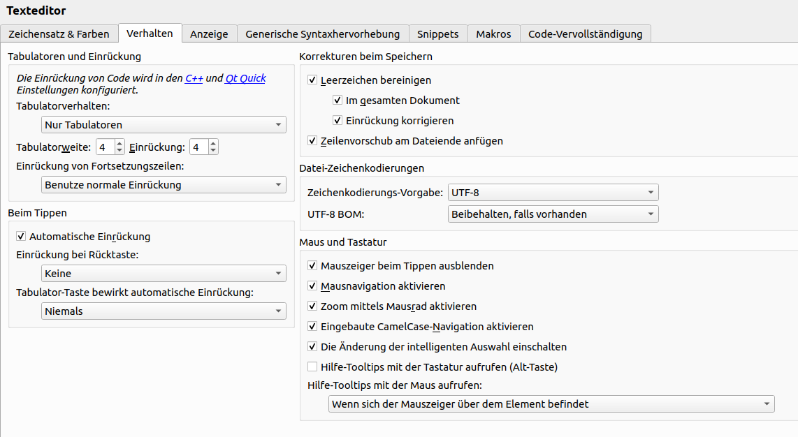
Please use the following Qt Creator text editor and coding style configuration. Some tipps on efficient Qt Creator use are given below.
2.3.1. TextEditor settings
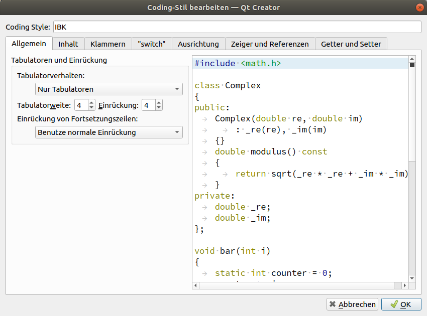
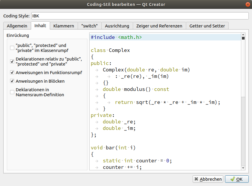
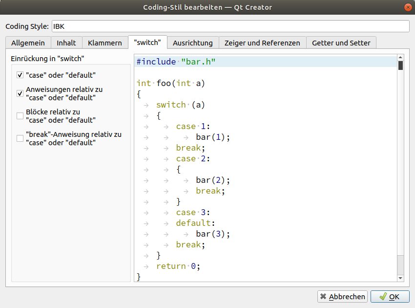
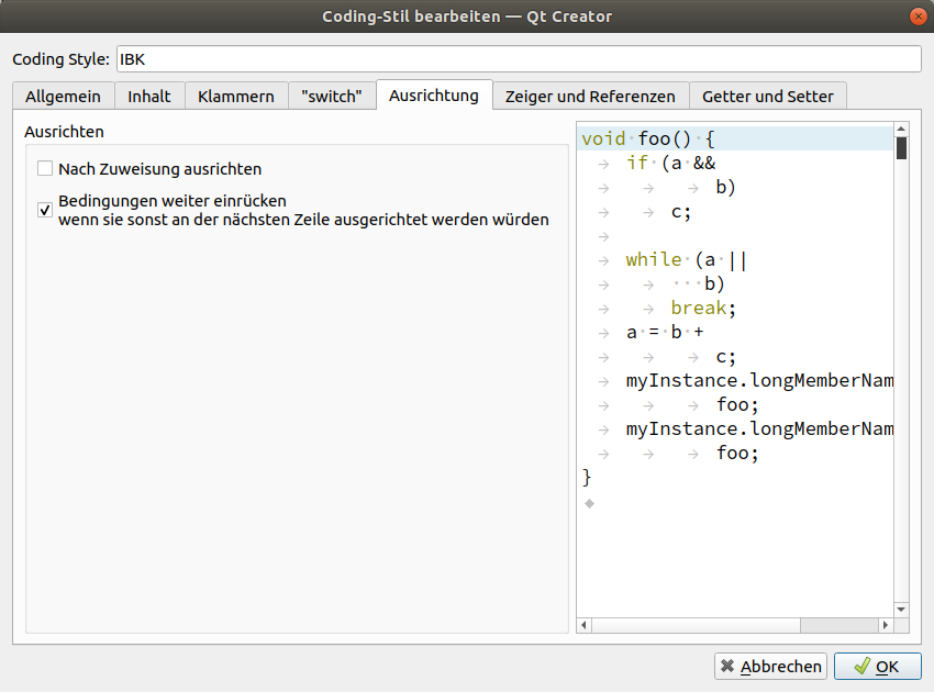
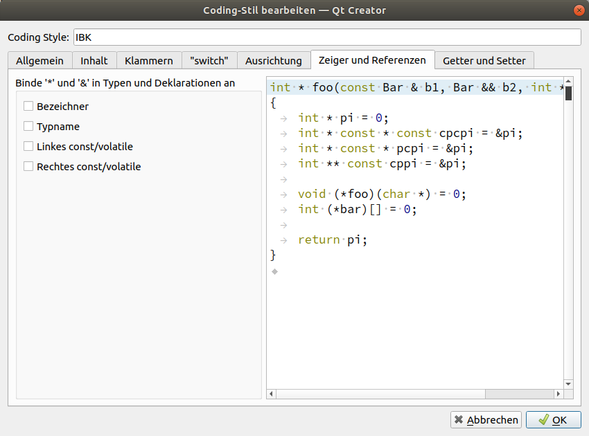
2.3.2. Coding style
Create a custom coding style (copy from Qt-style), name it "IBK" and change it as follows (not shown configuration pages need not be changed):
2.3.3. Other coding style settings:
-
C++ → Namenskonventionen für Dateien → Kleinbuchstaben für Dateinamen verwenden = off
2.3.4. Codemodel
The code model is responsible for checking the code while typing and can detect quite a few problems from mismatching types, misspelled variables, missing ; and basically everything a regular compiler can spot. In fact, the code model just runs the code through the first stages of the compiler - saving you quite a bit of compilation time.
The code model integration into Qt Creator is pretty nice, so you should activate it.
You can use one of the provided code model configurations, but that might lead to excessive number of errors/warnings. Rather configure the code model with the following parameters:
-Weverything -Wno-c++98-compat -Wno-c++98-compat-pedantic -Wno-unused-macros -Wno-newline-eof -Wno-exit-time-destructors -Wno-global-constructors -Wno-gnu-zero-variadic-macro-arguments -Wno-documentation -Wno-shadow -Wno-switch-enum -Wno-missing-prototypes -Wno-used-but-marked-unused -Wno-shorten-64-to-32 -Wno-old-style-cast
2.3.5. Efficient use of the Qt Creator IDE
-
Use F2 to lookup declaration/definitions of symbols (that means: variable, function declaration, type, …)
-
Use F4 to switch between header and cpp file
-
Use Shift-F4 to switch between UI-designer and h/cpp file
-
Ctrl+Shift+R - rename symbol using refacturing (i.e. everywhere that this symbol occurs in the source code)
-
"Alle Verweise" anzeigen im Kontextmenü (wenn man auf ein Symbol rechts-klickt)
Refactoring feature
See https://doc.qt.io/qtcreator/creator-editor-refactoring.html for a comprehensive list!
Make use of the refactoring feature (right-click on a symbol/variable/function/switch…) and select "Refacture" in the context menu.
Useful features are:
-
add definition in C++-File (when clicking on a function declaration)
-
add getter/setter functions (when clicking on a member variable with m_xxxYyyyZzzz naming)
-
complete switch clause (when clicking on a switch clause)
-
rename (Ctrl+Shift+R shortcut)
2.4. Code Quality
This section discusses a few techniques that help you write/maintain high quality code.
2.4.1. Frequently check for potential memory leaks
Use valgrind to check for memory leaks in regular intervals:
First run only initialization with --test-init flag.
> valgrind --track-origins=yes --leak-check=full ./NandradSolver /path/to/project --test-initYou should get an output like:
...
Stopping after successful initialization of integrator.
Total initialization time: 802 ms
==15560==
==15560== HEAP SUMMARY:
==15560==     in use at exit: 0 bytes in 0 blocks
==15560==   total heap usage: 3,776 allocs, 3,776 frees, 1,101,523 bytes allocated
==15560==
==15560== All heap blocks were freed -- no leaks are possible
==15560==
==15560== For counts of detected and suppressed errors, rerun with: -v
==15560== ERROR SUMMARY: 0 errors from 0 contexts (suppressed: 0 from 0)
Do this check with:
-
just the initialization part (i.e. with
--test-init) parameter -
run the initialization with some error in the input file to check if temporary variables during initialization are cleaned up correctly
-
also run a small part of the simulation, to check if something goes wrong during actual solver init and if tear-down is done correctly
-
run a small part of the simulation, then break (
Ctrl+C) and check if code cleanup after error abort is done correctly
|
Of course, in very flexible code structures as in NANDRAD solver, where many code parts are only executed for certain parameter combinations, checking all code variables for consistent memory allocation/deallocation is nearly impossible. Hence, writing safe code in the first place should be highest priority. |
Example: Avoiding memory leaks
NANDRAD creates model objects on the heap during initialization (never during solver runtime!). Since the model objects are first initialized before ownership is transferred, you should always ensure proper cleanup in case of init exceptions. Use code like:
ModelObject * modelObject = new ModelObject; // does not throw
m_modelContainer.push_back(modelObject); // transfer ownership, does not throw

modelObject->setup(...); // this may throw, but model object will be cleaned as part of m_modelContainer cleanup
If there is code between creation and ownership transfer, use code like:
std::unique_ptr<ModelObject> modelObject(new ModelObject);

modelObject->setup(...); // this may throw

m_modelContainer.push_back(modelObject.release()); // transfer ownership
2.4.2. Jacobian matrix pattern correctness check
It is easily possible to forget a specific interrelation and dependency when publishing model variable dependencies. The resulting sparse Jacobian-pattern may be incomplete.
An incomplete Jacobian-pattern has the following consequences:
-
The Newton-iteration may frequently not converge - the number of NonLinConvFails increases. Because of this, often a restart with new Newton-matrix setup and factorization is needed, which is expensive.
-
The Newton-iteration may converge, yet not entirely correct. This is picked up by the truncation error test, and leads potentially to an increase of ErrorFails and resulting step-rejections. Redoing a step is very bad for performance; time step is reduced, Jacobian matrix is recomputed and factorized… overall, the performance suffers.
-
The actual time to compose and factorize the Jacobian matrix may, however, be shorter when elements are missing. In some cases this can be desired, for example, when the Jacobian contains many very small values in its pattern. Then, it is often meaningful to drop these in the calculation. For example, the network interaction due to temperature-dependent viscosity changes may be omitted from the Jacobian. Also, the dependency of network element balance equations on a thermostat-controlled valve somewhere upstream reduces from element to element, until after several pipe segments the impact is no longer significant and could be dropped from the Jacobian.
Generally speaking, the Jacobian pattern should be complete and correct for most models, and this should be regularly checked.
Automatic consistency check
Under the condition that Jacobian matrixes for Dense and KLU are identical, the simulation should also run - theoretically - with identical results and solver statistics, only a bit slower in the case of the Dense matrix. Hence, it is a good first test to run the same test case with both matrix solvers and check, if there are significant differences.
When running a test case with the following options:
> NandradSolver test.nandrad --les-solver=Dense --integrator=ImplicitEuler -o="test.Dense"
> NandradSolver test.nandrad --les-solver=KLU -o="test.KLU"
this will generate two sets of output directories with (hopefully) identical physical results and statistics. However, even if the Jacobian pattern used by the sparse matrix solver is 100% correct, the rounding errors related to the LU factorization of the dense matrix, or the factorization of the re-arranged sparse matrix will likely give minor changes in the Newton solution which may accumulate over time and cause small differences in counters.
Still, the test can be done automated by running the script run_JacobianPatternTest.sh in the build/cmake directory.
|
Run the script |
The script will run all test cases with Dense and KLU solvers, compare results and statistics and flag all test cases with differences as failed.
Once a test case has been manually checked, a file with suffix jac_checked instead of nandrad can be placed side-by-side the NANDRAD project file. For all test cases with such a jac_checked file, the test will be skipped and the case will be marked as successful.
Manually checking Jacobian patterns
The sparse Jacobian pattern can be checked by comparing it against a full dense Jacobian matrix. If the sparse pattern is correct, the generated Jacobian matrixes must be identical, under the following conditions:
-
Jacobian matrix data is compared as originally computed in memory. Hence, dumping the data in binary format is required. When writing Jacobian data in ASCII format, there will be accuracy loss and hence small differences will be computed stemming from rounding errors.
-
Jacobian matrixes generated with DQ-algorithms must be generated using the same calculation method for the increments. For example, the increment calculation method in the SUNDIALS solvers is different from those in IBKMK-library - results will not be comparible. It is advised to use only IBKMK-matrix classes to generate Jacobian data.
-
All states must be identical, when the Jacobians are generated. This is usually only guaranteed at the begin of a simulation. Thus, the typical procedure is to generate the Jacobian, dump it to file and stop the solver right away.
-
The system function must be 100% deterministic and only dependent on the current set of states provided to the function. This also means that all embedded iterative/numerical algorithms must be started with exactly the same initial conditions. This applies, for example, to the Newton solver that is used for the hydraulic network calculation.
To generate the Jacobians to compare, the following changes need to be made in the solver’s source code:
|
Now you can generate the Jacobians for a specific test case using the command
> jacdump.sh test.nandradThis will run the test case with KLU and Dense (the latter with ImplicitEuler integrator) and then rename the dumped Jacobians to test_jacobian_dense.bin and test_jacobian_sparse.bin.
Now open these files with the JacobianMatrixViewer tool (see https://github.com/ghorwin/JacobianMatrixViewer).
If the matrixes match, you can run the script:
> checked.sh test.nandradwhich will create the test.jac_checked file and also remove the bin-files.
3. NANDRAD Solver
This chapter discusses the underlying fundamentals and algorithms, as well as initialization and calculation procedures.
3.1. Model Initialization Procedure
3.1.1. Pre-Solver-Setup steps
The following steps are done when initializing the model:
-
parsing command-line and handling early command line options
-
setting up directory structure and message handler/log file
-
creating
NANDRAD::Projectinstance -
setting default values via call to
NANDRAD::Project::initDefaults() -
reading the project file (only syntactical checks are done, and for IBK::Parameter static arrays with default units in keyword list, a check for compatible units is made), may overwrite defaults; correct units should be expected in the data model after reading the project file (maybe add suitable annotation to code generator?)
-
merge similarly behaving construction instances (reduce data structure size)
|
From now on the project data structure remains unmodified in memory until end of solver runtime and persistent pointers can be used to address parameter sets. This means no vector resizing is allowed, no more data members may be added/removed, because this would invalidate pointers/references to these vector elements. |
Error checking in NANDRAD data model
Some basic error checking can be made in the NANDRAD Project data structure that is independent of the actual simulation-dependend model setup. These tests are done in functions called checkParameters().
Basically, the NANDRAD Model calls these checkParameters() functions for all data objects. The functions should check for sane values (i.e. positive cross-section areas, non-negative coefficients, and generally all parameters with known limits. Also, the existence of parameters when required should be tested (in sofar this is independent of specific modelling options).
Error handling shall be done in such a way, that when parameter errors are found, the user can quickly identify the offending XML tag and fix the problem.
for (unsigned int i=0; i<m_project->m_materials.size(); ++i) {
	NANDRAD::Material & mat = m_project->m_materials[i];
	try {
		mat.checkParameters();
	}
	catch (IBK::Exception & ex) {
		throw IBK::Exception(ex, IBK::FormatString("Error initializing material #%1 '%2' (id=%3).")
							 .arg(i).arg(mat.m_displayName).arg(mat.m_id), FUNC_ID);
	}
}
Note, that in the exception the index, optional display name and ID is printed - one of these should be sufficient to find the problematic XML block.
The location of error is reported by the calling function, inside the checkParameters() function it is sufficient to indicate the actual parametrization error:
void Material::checkParameters() {
	// check for mandatory and required parameters and
	// check for meaningful value ranges
	m_para[P_Density].checkedValue("kg/m3", "kg/m3", 0.01, false, std::numeric_limits<double>::max(), true,
								   "Density must be > 0.01 kg/m3.");
	m_para[P_HeatCapacity].checkedValue("J/kgK", "J/kgK", 100, true, std::numeric_limits<double>::max(), true,
								   "Heat capacity must be > 100 J/kgK.");
	m_para[P_Conductivity].checkedValue("W/mK", "W/mK", 1e-5, true, std::numeric_limits<double>::max(), true,
								   "Thermal conductivity must be > 1e-5 W/mK.");
}
The exception hierarchy will be collected in the IBK::Exception objects and printed in the error stack (see also Exception handling).
For (the very frequently occurring) IBK::Parameter data type, the checkedValue() is most convenient to both check for existence and validity of an IBK::Parameter (including matching units). The function also returns the value in the requested target unit (see documentation for IBK::Parameter::checkedValue()).
Quick-access connections between data objects during runtime
Access of model parameters is very fast during simulation, if looping and searching through the data structure can be avoided. Pointers between data structures are an efficient way of relating data objects. For example, a construction layer references the respective material data via ID number of the material. During the initialization (specifically in checkParameters() a pointer is obtained to the material and stored in the object. This requires, of course, that the pointer may never become invalidated during the life-time of the simulation. Hence the strict requirement of not-changing vector sizes (see above).
If a references data element is missing, an error message is thrown (this is part of the reason, why this lookup of referenced data objects is done and checked in checkParameters().
Summary
-
implement
checkParameters()functions in NANDRAD data model classes -
for cross references between data members (via ID numbers of ID names), create fast access pointer links in this function
-
indicate the source of an error (i.e. the actual object) in the calling function
3.1.2. Model Setup
Now the actual model initialization starts.
TODO : model specific documentation
3.1.3. Climatic loads
Implementation
The Loads model is a pre-defined model that is always evaluated first whenever the time point has changed. It does not have any other dependencies.
It provides all resulting variables as constant (during iteration) result variables, which can be retrieved and utilized by any other model.
With respect to solar radiation calculation, during initialization it registers all surfaces (with different orientation/inclination) and provides an ID for each surface. Then, models can request direct and diffuse radiation data, as well as incidence angle for each of the registered surfaces.
Registering surfaces
Each construction surface (interface) with outside radiation loads registers itself with the Loads object, hereby passing the interface object ID as argument and orientation/inclination of the surface. The loads object itself registers this surface with the climate calculation module (CCM) and retrieves a surface ID. This surface ID may be the same for many interface IDs.
The Loads object stores a mapping of all interface IDs to the respective surface IDs in the CCM. When requesting the result variable’s memory location, this mapping is used to deliver the correct input variable reference/memory location to the interface-specific solar radiation calculation object.
3.2. Model objects, published variables and variable look-up
Physical models are implemented in model objects. That means the code lines/equations compute results based on input values.
A heating model takes room air temperature (state dependency) and a scheduled setpoint (time dependency) and computes a heating load as result.
The result is stored in a persistent memory location where dependent models can directly access this value.
3.2.1. Model instances
There can be several model instances - the actual object code resides only once in solver memory, but the functions are executed several times for each individual object (=model instance).
You may have a model that computes heat flux between walls and zones. For each wall-zone interface, an object is instantiated.
Each model instance stores its result values in own memory.
3.2.2. Model results
Publishing model results
The model instances/objects must tell the solver framework what kind of outputs they generate. Objects generating results must derive from class AbstractModel (or derived helper classes) and implement the abstract interface functions.
|
|
The framework first requests a reference type (prefix) via AbstractModel::referenceType() of the model object. This reference type is used to group model objects into meaningful object groups.
Typical examples are MRT_ZONE for zonal quantities, or MRT_INTERFACE for quantities (fluxes) across wall-surfaces.
Each invididual result variable is published by the model in an object of type QuantityDescription. The framework requests these via call to AbstractModel::resultDescriptions(). Within the QuantityDescription structure, the model stores for each computed quantity the following information:
-
id-name (e.g. "Temperature")
-
physical display unit (e.g. "C") - interpreted as "display unit", calculations are always done in base SI units
-
a descriptive text (e.g. "Room air temperature") (optional, for error/information messages)
-
physical limits (min/max values) (optional, may be used in iterative algorithms)
-
flag indicating whether this value will be constant over the lifetime of the solver/integration interval
|
A note on units
The results are stored always in base SI units according to the IBK-UnitList. A well-behaving model will always store the result value in the basic SI unit, that is "K" for temperatures, "W" for thermal loads and so on (see |
The unit is really only provided for error message outputs and for checking of the base SI unit matches the base SI unit of the requested unit (as an additional sanity check).
Vector-valued results
Sometimes, a model may compute a vector of values.
A ventilation model may compute ventilation heat loads for a number of zones (zones that are identified via object lists).
When a so-called vector-valued quantity is generated, the following additional information is provided:
-
whether index-based or id-based access is anticipated
-
a list of ids/indexes matching the individual positions in the vector (the size of the vector is also the size of the vector-valued quantities)
The aforementioned ventilation model may be assigned to zones with IDs 1,4,5,10 and 11. Then the resulting ventilation heat losses will be defined for those zones only. Hence, the published quantity will look like:
- name = "NaturalVentilationHeadLoad"
- unit = "W"
- description = "Natural ventilation heat load"
- index-key-type = "ID"
- ID-list = {1,4,5,10,11}|
Strong uniqueness requirement
The id-names of quantities are unique within a model object, and vector-valued quantities may not have the same ID name as scalar quantities. More precisely, variables need to be globally unique (see lookup rules below). This means that when there are two models with the same model-reference-type, the variable names must be unique among all models with the same reference-type. For example: from a zone parametrization several models are instantiated with the same reference-type |
Initializing memory for result values
Each model object is requested by the framework in a call to AbstractModel::initResults() to reserve memory for its result variables. For scalar variables this is usually just resizing of a vector of doubles to the required number of result values. For vector-valued quantities the actual size may only be known later, so frequently here just the vectors are created and their actual size is determined later.
|
Since the information collected in |
Convenience implementation
Scalar variables are stored in double variables of the model. When using the convenience implementation in DefaultModel these are stored in vector m_results.
Vector-valued variables are stored in consecutive memory arrays with size matching the size of the vector. When using the DefaultModel implementation, these are stored in m_vectorValuedResults, which is a vector of VectorValuedResults.
The DefaultModel implementation makes use of enumerations Results and VectorValuedResults.
3.2.3. Model inputs
Similarly as output variables, model objects need input variables. Models requiring input must implement the interface of class AbstractStateDependency.
Input variable requirements are published similarly to results when the framework requests them in a call to AbstractStateDependency::inputReferences(). The information on requested results is stored in objects of type InputReference. The data in class InputReference is somewhat similar to that of QuantityDescription but contains additional data regarding the expectations of the model in the input variable.
|
A model may request scalar variable inputs only, even if the providing model generates these as a vector-valued quantity. That means, a model has the choice to request access to the entire vector-valued variable (and will usually get the address to the start of the vector-memory space), or a single component of the vector. In the latter case, the index/model-ID must be defined in the |
An input required by the ventilation model can be formulated with the follwing data:
- reference type = MRT_ZONE
- object_id = 15 (id of the zone)
- name = "AirTemperature"
Given that information, the framework can effectively look-up the required variables.
Once the variable has been found, the framework will tell the object the memory location by calling AbstractStateDependency::setInputValueRef().
FMI Export (output) variables
When FMI export is defined, i.e. output variables are declarted in the FMI interface, a list of global variable IDs to be exported is defined. For each of these variables an input reference is generated (inside the FMIInputOutput model), just as for any other model as well.
Suppose an FMI exports the air temperature from zone id=15 and for that purpose needs to retrieve the currently computed temperature from the zone state model. The FMI output variable would be named Zone[15].AirTemperature and the input reference would be created as in the example above. This way, the framework can simply provide a pointer to this memory slot to the FMIInputOutput model just as for any other model.
Outputs
When initializing outputs, any published variable can be collected. Outputs declare their input variables just as any other model object.
3.2.4. Variable lookup
The frameworks job is to collect all
Resolving persistant pointers to result locations
Later, when the framework connects model inputs with results, the framework requests models to provide persistant memory locations for previously published results. This is done by calling AbstractModel::resultValueRef(), which get’s a copy of the previously exported InputReference.
In order to uniquely identify a result variable within a model, normally only two things are needed:
-
the ID name of the variable,
-
and, only in the case of vector-valued quantities, the index/id.
However, in some cases, a model may request a variable with the same quantity name, yet from two different objects (for example, the air temperature of neighbouring zones). In this case, the quantity name alone is not sufficient. Hence, the full input reference including object ID is passed as identifier (A change from NANDRAD 1!).
|
To identify an element within a vector-valued result it is not necessary to specify whether it should be index or id based - the model publishing the result defines whether it will be index or id based access. |
Naturally, for scalar result variables the index/id property is ignored.
The QuantityName struct contains this information (a string and an integer value).
Now the model searches through its own results and tries to find a matching variable. In case of vector-valued quantities it also checks if the requested id is actually present in the model, and in case of index-based access, a check is done if the index is in the allowed range (0…size-1).
If a quantity could be found, the corresponding memory address is returned, otherwise a nullptr. The framework now can take the address and pass it to any object that requires this input.
Global lookup rules/global variable referencing
To uniquely reference a resulting variable (and its persistent memory location), first the actual model object/instance need to be selected with the following properties:
-
the type of object to search for (= reference-type property), for example
MRT_ZONEorMRT_CONSTRUCTIONINSTANCE -
ID of the referenced object, i.e. zone id oder construction id.
Some model objects exist only once, for example schedules or climatic loads. Here, the reference-type is already enough to uniquely select the object.
Usually, the information above does select several objects that have been created from the parametrization related to that ID. For example, the zone parameter block for some zone ID generates several zone-related model instances, all of which have the same ID. Since their result variables are all different, the framework simply searches through all those objects until the correct variable is found. These model implementations can be thought of as one model whose equations are split up into several implementation units.
The actual variable within the selected object is found by ID name and optionally vector-element id/index, as described above.
The data is collected in the class InputReference:
-
ObjectReference( holds reference-type and referenced-object ID ) -
QuantityName(holds variable name and in case of vector-valued quantities also ID/index)
Also, it is possible to specify a constant flag to indicate, that during iterations over cycles the variable is to be treated constant.
|
If several model objects are addressed by the same reference-type and ID (see example with models from zone parameter block), the variable names must be unique among all of these models. |
FMI Input variable overrides
Any input variable requested by any other model can be overridden by FMU import variables. When the framework looks up global model references, and an FMU import model is present/parametrized, then first the FMI generated quantity descriptions are checked. The FMU import variables are exported as global variable references (with ObjectReference). Since these are then the same global variable identifiers as published by the models, they are found first in the search and dependent models will simply store points to the FMU variable memory.
Examples for referenced input quantities
Setpoint from schedules
Schedules are defined for object lists. Suppose you have an object list name "Living rooms" and corresponding heating/cooling setpoints.
Now a heating model may be defined that computes heating loads for a given zone. The heating model is implemented with a simple P-controller, that requires zone air temperature and zone heating setpoint.
Definition of the input reference for the zone air temperature is done as in the example above. The setpoint will be similarly referenced:
- reference type = MRT_ZONE
- object_id = 15 (id of the zone)
- name = "HeatingSetPoint"
4. SIM-VICUS User-Interface
4.1. 3D Engine
4.1.1. Camera
-
world-2-view-translation = m_projection * m_camera * m_transform
-
transform only for "movable objects" (e.g. objects in selection)
-
Local coordinate system of camera = left handed coordinate system with y-axis pointing downwards and z-axis pointing towards user
+ right = towards right of screen
+ up = pointing downwards
+ forward = towards the viewer
-
camera object without translation and rotation → x and y coordinates map to i-j coordinates of screen (0,0 top left; 1,1 bottom right), so that point x,y,z = (-50,-200,0) becomes i,j = (-100, 400) (bottom left) in screen coordinates.
4.1.2. Navigation
Die Kamera kann mittels Tastatur- und Mauseingaben verschoben und gedreht werden.
Tastaturnavigation erfolgt mit den Tasten W, A (Vor- und Zurück), S, D (nach links, nach rechts verschieben), R, F (hoch oder runter verschieben), Q, E (links oder rechts um die globale Z-Achse drehen).
Mit der Maus sind 4 verschiedene Operationen möglich:
-
First-Persion-View-Modus: beim Halten der rechten Maustaste führt die Mausbewegung um einen Kameraschwenk um die Kameraposition
-
Verschieben der Kamera: beim Halten der mittleren Maustaste wird die Kamera so verschoben, sodass der angeklickte Punkt unter dem Cursor bleibt.
-
Orbit-Modus: beim Halten der linken Maustaste bewegt und rotiert sich die Kamera um den angeklickten Punkt.
-
Schneller Vor-/Zurück-Modus: beim Bewegen des Scroll-Rads bewegt sich die Kamera schnell vor/zurück entlang der aktuellen Sichtrichtung. Ist gleichzeitig die linke Maustaste gedrückt, so bewegt sich die Kamera entlang der Sichtline auf den angeklickten Punkt zu.
Die Operation 1-3 sind exclusive, d.h. man kann stets nur eine gleichzeitig ausführen.
4.1.3. Data transfer
-
original geometry in object coordinates (world coordinate for now)
-
opaque geometry = planes
Primitive Assembly
-
planes:
-
type triangle
-
type rect
-
type polygon
-
-
plane type affects selection algorithm: triangle/rect trivial; polygon = test individual triangles (more work)
-
data on VBO first stored on heap (vector of vertex struct); additional vector for rgba colors
-
plane transfer vectors, type-specific transfer:
-
append vertices + colors
-
store element indexes in triangle-strip order
-
append primitive restart index, see https://www.khronos.org/opengl/wiki/Vertex_Rendering#Primitive_Restart
-
-
triangles: copy 3 vertices counter-clock-wise; append element indexes +0, +1, +2
-
rectangle: copy 4 vertices counter-clock-wise; append element indexes +0, +1, +2; +1 +3 +2
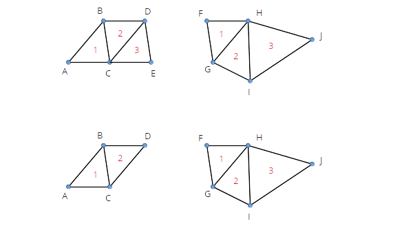
Triangle Strips
See also explanation in https://www.learnopengles.com/tag/triangle-strips.
See polygon in Figure 3. Index list to draw the polygon is:
1, 2, 6, 5, 3, 4
-
First triangle is
1, 2, n(anti-clock-wise - order of first triangle defines order of the rest). -
Second triangle is
2, n-1, n -
Third triangle is
n, 3, n-1 -
Fourth triangle is
3, n-2, n-1-
in an algorithm keep adding indexes until you would duplicate an existing node index
-
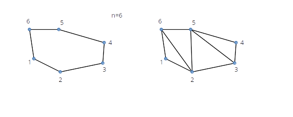
When drawing several triangle strips one after another, we need primitive restart (to have gaps between triangles).
Consider strips in Figure 4. Top part of the figure shows two strips where the first strip ends with an odd numbered triangle. Bottom part shows the first strip ending with an even numbered triangle.
4.1.4. Shaders
Vertex-Layout notation:
-
V - single coordinate (e.g. x-coordinate)
-
N - component of normal vector
-
C - color component (e.g. CCC for RGB)
-
T - texture coordinate
Grid
-
Shader-Index: 0
-
Vertex-Structure: (VV) = (xz)
-
Files:
grid.vertandgrid.frag -
Uniforms (variables):
-
worldToView -
gridColor -
backColor(fade-to color) -
(optional)
farDistance(fade-to normalization distance)
-
Background Objects
Uniform color, no lighting effect, no transparency
-
Shader-Index: 1
-
Vertex-Structure: (VVVCCC) = (xyzrgb)
-
Files:
vertexColor.vertandflat.frag -
Uniforms (variables):
-
worldToView
-
Regular Opaque Objects
-
Shader-Index: 2
-
Vertex-Structure: (VVVNNNCCC) = (xyzNxNyNzrgb)
-
Files:
vertexNormalColor.vertandspecularShading.vert -
Uniforms (variables):
-
worldToView -
lightPos
-
4.2. 3D Calculations
This chapter describes/discusses many of the unterlying 3D geometry calculations used in SIM-VICUS.
|
We are dealing with limited number precision when performing geometry calculations. Hence, when checking for same vertexes, collinearity, and many other properties we need to deal with a little bit of fuzzyness. For example, the vertexes (0,1,0) and (1e-4, 0.9999, -1e.4) should be treated the same. Generally speaking, we need to define a (problem specific) relative and absolute tolerance to be used when comparing geometrical properties. However, in the implementation we often use comparisons with cached variables to avoid updates when no changes have been made. In these comparisons we need to check for exactly the same values. |
4.2.1. Polygons
Polygons are defined through lists of vertexes. There can be valid and invalid polygons.
Valid polygons
Valid polygons have the following properties:
-
there are at least 3 vertexes
-
all vertexes must lie in a plane (within given tolerance limit)
-
all vertices are different (within given tolerance limit)
-
two subsequent edges are not collinear (within given tolerance limit)
-
polygon is not winding (i.e. no two edges cross)
Reducing vertex lists to get valid polygons
When drawing a polygon or starting with a given set of vertexes, we can remove vertexes that would violate any of the rules above in the following manner:
-
remove subsequent vertexes which are the same
-
compute edge direction vectors, and if two adjacent edge direction vectors are collinear, remove the middle vertex
4.2.2. Normal vector calculation of polygons
Polygons are expected to be not-winding and defined in counter-clockwise manner. Then, the normal vector of the polygon can be created by computing the cross product of two adjacent edges. However, if polygons are concave, the sign of the normal vector depends on the edge being selected. Figure 5 shows a concave polygon.

Suppose the following vertex coordinates define the polygon:
1:   4,0,0
2:   2,2,0
3:   4,3,0
4:   0,4,0
5:   0,0,0
If we select vertexes 1, 2 and 3 and compose the cross product of the enclosed edges, we get:
a = v1-v2 = (2,-2,0)
b = v3-v2 = (2,1,0)
n = a x b = (0,0,6) (pointing upwards)
If we select vertexes 2, 3 and 4 we get:
a = v2-v3 = (-2,-1,0)
b = v4-v3 = (-4,1,0)
n = a x b = (0,0,-6)  (pointing downwards)
So, just picking a random point and computing the cross product between the adjacent edges does not work.
Since we do a triangulation for any valid polygon anyways (needed for drawing purposes), we can then easily just take any of the generated triangles and compute the normal of the triangle (all triangles will have the same normal vector).
|
We actually need to compute the normal vector already before we have a triangulation: for checking if all vertexes lie in a plane. However, for this check the sign of the normal vector is of no importance, and once the triangulation has been computed, we just update the normal vector with the correct one. |
4.3. Zustand der Benutzeroberfläche (View State)
Die Benutzeroberfläche hat verschiedene Zustände, wobei ein Zustand beschreibt:
-
welche Ansicht ein Widget zeigt, z.B. welches Property-Widget gerade aktiv/sichtbar ist
-
welche Maus-/Tastaturinteraktionsmöglichkeiten bestehen, z.B. was die linke Maustaste bewirkt oder welche Snap-Funktionen eingeschaltet sind
-
was die Szene anzeigt (z.B. lokales Koordinatensystem sichtbar oder nicht)
Da das Verändern eines Zustands mehrere Teile der Oberfläche (und damit mehrere Objekte)
betrifft, wird das Ändern des Oberflächenzustands zentralisiert über einen
Zustandsmanager (SVViewStateHandler) erledigt.
Beim Setzen eines neuen Zustands sendet dieser ein Signal aus.
Alle Widgets/Objekte, die sich in Abhängigkeit des Zustands verändern müssen, sollten auf dieses Signal reagieren und sich entsprechend anpassen.
Eine Veränderung des Zustands kann überall in der Programmoberfläche ausgelöst werden und erfolgt in folgenden Schritten:
-
holen des aktuellen Zustands (Objekt
ViewState) -
anpassen des Zustandsbeschreibungsobjekts
-
setzen des neuen Zustands
// aktuellen ViewState holen
ViewState vs = SVViewStateHandler::instance().viewState();
// anpassen
vs.m_sceneOperationMode = OM_SelectedGeometry;
vs.m_propertyWidgetMode = PM_EditGeometry;
// setzen
SVViewStateHandler::instance().setViewState(vs);
4.3.1. ViewMode
Umschalten erfolgt durch Modusauswahl-Schaltflächen in der linken Toolbar
-
VM_GeometryEditMode- wenn Geometrie bearbeitet wird; Geometrie wird mit definierten Oberflächen/Materialfarben dargestellt -
VM_PropertyEditMode- beim Eigenschaften ansehen/bearbeiten; Geometrie wird mit Falschfarben je nach Modus dargestellt
Beim Umschalten zwischen den Modi wird die Geometrie neu eingefärbt und gezeichnet.
Im VM_PropertyEditMode: NUM_OM + NUM_L und PropertyWidgetMode wird je nach Auswahl im SVPropModeSelectionWidget gesetzt, genau wie
ObjectColorMode.
(ACHTUNG: Shortcuts zum Ändern des SceneOperationMode deaktivieren!)
Beim Einschalten des VM_GeometryEditMode wird unterschieden:
-
Es gibt eine Auswahl von Flächen, dann:
OM_SelectedGeometry+PM_EditGeometry-
4.4. Auswahl von Objekten
Wenn die Benutzeroberfläche im Zustand:
-
Standard (NUM_OM)
-
OM_SelectedGeometry
ist, kann man Objekte durch links-klicken auswählen. Alternativ kann man im Navigationsbaum auswählebare Objekte durch Ankreuzen der Auswahlboxen auswählen.
4.4.1. Auswahl in der Scene
Wenn ein Linksklick registriert wird, werden alle geometrischen Primitiven auf Kollision mit der Sichtgeraden geprüft und ggfs. selektiert/deselektiert. Dies erfolgt in der Funktion Vic3DScene::handleSelection().
Hier wird zunächst die "pick"-Operation durchgeführt, wobei der Sichtstrahl konstruiert und die Kollisionsprüfung mit allen Objekten durchgeführt wird. Ist ein Objekt ermittelt, wird dieses eindeutig durch seinen uniqueID identifiziert. Alle Objekte im Navigationsbaum müssen eine solche haben, und sind deshalb von VICUS::Object abgeleitet. Diese Klasse speichert auch das "selected"-Flag.
Wurde ein Objekt angeklickt, wird eine Undo-Action vom Typ SVUndoTreeNodeState erstellt. Diese sammelt zunächst basierend auf der übergebenen uniqueID alle zu verändernden Elemente aus.
4.5. Objekt-Pick-Operation
Die Erkennung, was sich unter dem Mauscursor befindet, kann unterschiedliche Ergebnisse haben, je nach Konfiguration. Dafür wird zunächst ein PickObject erstellt und konfiguriert und dann dem Pick-Algorithmus übergeben.
Optionen sind:
-
XY_Plane- es wird ein Schnittpunkt mit der XY-Ebene bestimmt -
Surface- es werden alle Oberflächen geprüft -
Network- es werden Netzwerkobjekte (Nodes/Edges) geprüft -
Backside- es werden auch die Rückseiten von Objekten geprüft
5. NANDRAD FMU
5.1. Debugging NANDRAD FMUs mit Qt Creator und MasterSim
5.1.1. Linux
-
MasterSim von SourceForge herunterladen
oder
-
MasterSim-Repository von SourceForge herunterladen und mit CMake kompilieren
|
Es wird ein statisch gelinktes |
Aufsetzen der Co-Simulation
-
Ein Co-simulationsprojekt in MasterSim erstellen und speichern, beispielsweise unter
/home/ghorwin/git/SIM-VICUS/data/fmu/coSimulation.msim -
einmal mit MasterSimulator ausführen:
> /path/to/MasterSimulator /home/ghorwin/git/SIM-VICUS/data/fmu/coSimulation.msimDies erstellt die übliche Verzeichnisstruktur unter: /home/ghorwin/git/SIM-VICUS/data/fmu/coSimulation.msim.
Qt-Creator für das FMU-Debuggen konfigurieren
-
Qt Creator öffnen
-
Modus "Projekte" öffnen
-
In der Rubrik "Ausführen", in der Zeile mit "Ausführungskonfiguration" (da steht normalerweise SIM-VICUS oder NandradSolver drin) auf "Add…" klicken
-
In der Liste "Benutzerdefinierte ausführbare Datei" anklicken und bestätigen → es wird eine neue Ausführungskonfiguration erstellt.
-
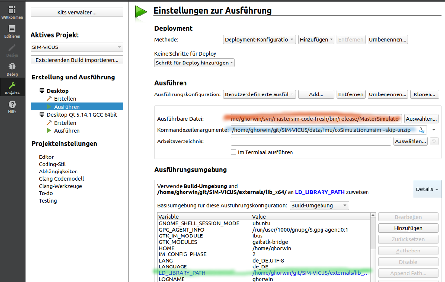
Wie in der Abbildung oben zu sehen eintragen:
-
(rot) Pfad zum MasterSimulator Programm
-
(blau) Pfad zur
msim-Projektdatei und zusätzlich das Argument--skip-unzip
-
-
Dann unten bei der Ausführungsumgebung die Details ausklappen
-
Die Umgebungsvariable
LD_LIBRARY_PATHhinzufügen, und als Wert den Pfad zumSIM-VICUS/externals/lib_x64:Pfad eintragen; MasterSim muss beim Laden der FMU-Bibliothek alle von ihr gelinkten, dynamischen Bibliotheken finden.
Jetzt kann man den Debugger starten (F5) und man müsste MasterSim durchlaufen sehen.
|
Trotz der Angabe von
|
Wenn man im QtCreator irgendwo einen Breakpoint setzt, und dann in der Debugger-Module-Ansicht die geladenen Shared Libraries ansieht, kann man diesen Pfad wiederfinden.
Beispiel:
-
MasterSim Projekt:
/home/ghorwin/git/SIM-VICUS/data/fmu/coSimulation.msim -
Lib-Pfad:
/home/ghorwin/git/SIM-VICUS/externals/lib_x64/
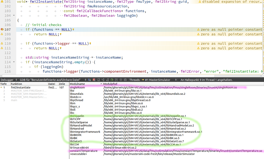
fmi2Instantiate-
(rosa) Im Bild rosa markiert sind die geladenen FMUs im Co-Simulationsszenario.
-
(grün) Im Bild grün markiert sind die davon abhängigen Bibliotheken
|
Es kann jetzt sein, dass die FMU-Bibliothek im |
Debuggen der aktuellen Entwicklungsversion
Löscht man die "alte" FMU Bibliothek aus dem binaries/linux64-Verzeichnis erhält man eine Fehlermeldung, z.B.
Shared library '/home/ghorwin/git/SIM-VICUS/data/fmu/coSimulation/fmus/singleRoom/binaries/linux64/singleRoom.so' does not exist.
Man erstellt nun einen Symlink auf die aktuell entwickelte FMU-Bibliothek an Stelle der originalen FMU-Bibliothek, welche von MasterSim geladen wird.
Im Verzeichnis: /home/ghorwin/git/SIM-VICUS/data/fmu/coSimulation/fmus/singleRoom/binaries/linux64/:
ln -s /home/ghorwin/git/SIM-VICUS/bin/debug_x64/libNandradSolverFMI.so singleRoom.soDies erstellt eine symbolische Verknüpfung zur gerade entwickelten Bibliothek libNandradSolverFMI.so.
Wenn man nun den Debugger startet, lädt MasterSim stattdessen diese aktuelle Bibliothek. Damit der symbolische Link nicht wieder überschrieben wird, muss das Argument --skip-unzip verwendet werden.
Nun kann man die FMU ganz normal debuggen.
6. Patches/Diffs
6.1. Änderungen in abgeleiteten Projekten übernehmen
6.1.1. Ausgangspunkt
Es gibt eine VICUS oder NANDRAD Projektdatei im ASCII-Format. Es werden davon mittels Texteditor modifizierte Versionen erstellt, Beispiel:
# Original
Reihenhaus_Basis.nandrad
# Variante mit Fußbodenheizung
Reihenhaus_Fussbodenheizung.nandrad
# Variante mit FMU Interface B1
B1_Reihenhaus_Fussbodenheizung_FMI.nandrad
Die Änderungen zwischen zwei Dateiversionen lassen sich grafisch z.B. mit meld oder kompare anzeigen:
> meld Reihenhaus_Basis.nandrad Reihenhaus_Fussbodenheizung.nandrad
# oder
> kompare Reihenhaus_Basis.nandrad Reihenhaus_Fussbodenheizung.nandrad
Die Änderung von Datei 1 zu 2 lassen sich mit dem Befehl:
> diff -U 3 -dHrN -- Reihenhaus_Basis.nandrad Reihenhaus_Fussbodenheizung.nandradals diff vereinigt in der Konsole anzeigen, z.B.:
--- Townhouse_reference_210609.nandrad	2021-06-11 14:54:46.000000000 +0200
+++ B1_Townhouse_1_210614.nandrad	2021-06-11 15:47:29.000000000 +0200
@@ -351,6 +351,7 @@
 				</MaterialLayers>
 			</ConstructionType>
 			<ConstructionType id="20006" displayName="[FMI4BIM] Town house Floor Upper Floor">
+			<ActiveLayerIndex>1</ActiveLayerIndex>
 				<MaterialLayers>
 					<MaterialLayer thickness="0.015" matId="10017" />
 					<MaterialLayer thickness="0.065" matId="10019" />
@@ -424,15 +425,29 @@
 						</DailyCycles>
 					</Schedule>
 				</ScheduleGroup>
+				<ScheduleGroup objectList="[FMI4BIM] Townhouse Adapter">
+					<Schedule type="AllDays">
+						<DailyCycles>
+							<DailyCycle interpolation="Constant">
+								<TimePoints>0</TimePoints>
+								<Values>FluidOutletSetpointSchedule [C]:40</Values>
+							</DailyCycle>
+							<DailyCycle interpolation="Constant">
+								<TimePoints>0</TimePoints>
+								<Values>SupplyMassFlowSchedule [kg/s]:0.05</Values>
+							</DailyCycle>
+						</DailyCycles>
+					</Schedule>
+				</ScheduleGroup>
 			</ScheduleGroups>
 		</Schedules>
 		<Models>
 			<NaturalVentilationModels>
-				<NaturalVentilationModel id="4" displayName="[FMI4BIM] Townhouse ZoneTemplate Living Space" modelType="Constant">
+				<NaturalVentilationModel id="5" displayName="[FMI4BIM] Townhouse ZoneTemplate Living Space" modelType="Constant">
 					<ZoneObjectList>[FMI4BIM] Townhouse ZoneTemplate Living Space</ZoneObjectList>
 					<IBK:Parameter name="VentilationRate" unit="1/h">0.65</IBK:Parameter>
 				</NaturalVentilationModel>
-				<NaturalVentilationModel id="5" displayName="[FMI4BIM] Townhouse ZoneTemplate Roof" modelType="Constant">
+				<NaturalVentilationModel id="6" displayName="[FMI4BIM] Townhouse ZoneTemplate Roof" modelType="Constant">
 					<ZoneObjectList>[FMI4BIM] Townhouse ZoneTemplate Roof</ZoneObjectList>
 					<IBK:Parameter name="VentilationRate" unit="1/h">1.1</IBK:Parameter>
 				</NaturalVentilationModel>
@@ -453,13 +468,29 @@
 					<ControllerType>Analog</ControllerType>
 				</Thermostat>
 			</Thermostats>
-			<IdealHeatingCoolingModels>
-				<IdealHeatingCoolingModel id="3">
-					<ZoneObjectList>[FMI4BIM] Townhouse ZoneTemplate Living Space</ZoneObjectList>
+			<IdealSurfaceHeatingCoolingModels>
+				<IdealSurfaceHeatingCoolingModel id="3">
+					<ThermostatZoneId>13</ThermostatZoneId>
+					<ConstructionObjectList>[FMI4BIM] Townhouse Ground Floor</ConstructionObjectList>
 					<IBK:Parameter name="MaxHeatingPowerPerArea" unit="W/m2">50</IBK:Parameter>
-					<IBK:Parameter name="MaxCoolingPowerPerArea" unit="W/m2">0</IBK:Parameter>
-				</IdealHeatingCoolingModel>
-			</IdealHeatingCoolingModels>
+				</IdealSurfaceHeatingCoolingModel>
+				<IdealSurfaceHeatingCoolingModel id="4">
+					<ThermostatZoneId>14</ThermostatZoneId>
+					<ConstructionObjectList>[FMI4BIM] Townhouse Upper Floor</ConstructionObjectList>
+					<IBK:Parameter name="MaxHeatingPowerPerArea" unit="W/m2">50</IBK:Parameter>
+				</IdealSurfaceHeatingCoolingModel>
+			</IdealSurfaceHeatingCoolingModels>
+			<HeatLoadSummationModels>
+				<HeatLoadSummationModel id="7">
+					<ObjectList>All constructions</ObjectList>
+				</HeatLoadSummationModel>
+			</HeatLoadSummationModels>
+			<NetworkInterfaceAdapterModels>
+				<NetworkInterfaceAdapterModel id="8" summationModelId="7">
+					<IBK:Parameter name="FluidHeatCapacity" unit="J/kgK">4180</IBK:Parameter>
+				</NetworkInterfaceAdapterModel>
+			</NetworkInterfaceAdapterModels>
+
 		</Models>
 		<Outputs>
 			<Definitions>
@@ -468,6 +499,41 @@
 					<ObjectListName>All zones</ObjectListName>
 					<GridName>Hourly values</GridName>
 				</OutputDefinition>
+				<OutputDefinition>
+					<Quantity>ActiveLayerThermalLoad</Quantity>
+					<ObjectListName>All constructions</ObjectListName>
+					<GridName>Hourly values</GridName>
+				</OutputDefinition>
+				<OutputDefinition>
+					<Quantity>VentilationHeatLoad</Quantity>
+					<ObjectListName>All zones</ObjectListName>
+					<GridName>Hourly values</GridName>
+				</OutputDefinition>
+				<OutputDefinition>
+					<Quantity>ConstructionHeatConductionLoad</Quantity>
+					<ObjectListName>All zones</ObjectListName>
+					<GridName>Hourly values</GridName>
+				</OutputDefinition>
+				<OutputDefinition>
+					<Quantity>WindowHeatConductionLoad</Quantity>
+					<ObjectListName>All zones</ObjectListName>
+					<GridName>Hourly values</GridName>
+				</OutputDefinition>
+				<OutputDefinition>
+					<Quantity>WindowSolarRadiationLoad</Quantity>
+					<ObjectListName>All zones</ObjectListName>
+					<GridName>Hourly values</GridName>
+				</OutputDefinition>
+				<OutputDefinition>
+					<Quantity>TotalHeatLoad</Quantity>
+					<ObjectListName>Summation</ObjectListName>
+					<GridName>Hourly values</GridName>
+				</OutputDefinition>
+				<OutputDefinition>
+					<Quantity>ReturnTemperature</Quantity>
+					<ObjectListName>[FMI4BIM] Townhouse Adapter</ObjectListName>
+					<GridName>Hourly values</GridName>
+				</OutputDefinition>
 			</Definitions>
 			<Grids>
 				<OutputGrid name="Hourly values">

 				... <Rest abgeschnitten>...
Die Ausgabe lässt sich in eine Datei umleiten:
> diff -U 3 -dHrN -- Reihenhaus_Basis.nandrad Reihenhaus_Fussbodenheizung.nandrad > patch-zuFussbodenheizung.diffWird nun die originale Datei verändert, z.B. als Reihenhaus_Basis_v1.nandrad gespeichert, kann man die Änderungen erneut anwenden:
> patch Reihenhaus_Basis_v1.nandrad patch-zuFussbodenheizung.diffHierbei wird die Datei Reihenhaus_Basis_v1.nandrad verändert.
Das Ganze lässt sich geskriptet benutzen, um eine Reihe von aufeinander aufbauenden Dateien zu patchen.
|
Um Datenverlust bei Patchkonflikten zu vermeiden, sollte man das betreffende Verzeichnis und die zu patchenden Dateien in ein git-Repository einpacken, sodass man zur Not die Änderungen rückgängig machen kann. |